
An exploration of volatility modelling within the HJM framework using PCA on UK forward rate data. The study estimates dominant factors driving yield curve movements and discusses implications for no-arbitrage modelling.
Introduction
The Heath-Jarrow-Morton (HJM) framework allows practitioners to model the term structure of interest rates via the stochastic evolution of forward rates. This approach contrasts with traditional short-rate models which focus on the spot rate and derive the yield curve from it. In this discussion, we present an informal overview of the HJM Framework and then apply Principal Component Analysis (PCA) to initiate the estimation of a volatility structure.
Part 1 Theoretical Underpinnings and Derivations
1.1 Intuition for the Instantaneous Forward Rate
We are concerned with modelling the entire term structure of interest rates. To enable this, we consider the behaviour of forward rates and particularly the instantaneous forward rates.
Forward Rate

Denotes the interest rate quoted at time t for the period commencing at time T1 and maturing at time T2
We can then define the instantaneous forward rate at time T by considering the limit when the holding period approaches zero.
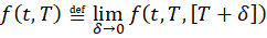
This is a theoretical tool in which we start by considering that, at time t, we agree to lend money to be returned at time T + Δ. As we let Δ approach zero, the idea is to capture the behaviour of lending over an infinitesimally small time interval. While it’s not possible in practice to lend or borrow over such a short period it remains a useful theoretical concept as it provides the foundation for deriving and analysing the yield curve.
1.2 Relationship to Bond Price

This price is critical as it reflects the present value of receiving a unit of currency at time T. Mathematically, the bond price is related to the instantaneous forward rate by the following expression.
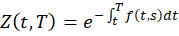
Economically, the equation above represents the discounting of the future cash flow of the bond by continuously compounding the corresponding forward rates over the interval [ t , T ].Consequently, by modelling the instantaneous forward rate we can reconstruct the yield curve allowing us to price any zero-coupon bond and by extension any interest rate product.
1.3 Dynamics
Under the HJM framework, the dynamics of the instantaneous forward rate are assumed to be given by the stochastic differential equation below.

\text{Where } \alpha(t,T) \text{ and } \sigma(t,T) \text{ are stochastic processes adapted to the filtration } \{\mathcal{F}_t\}_{t \geq 0}, \text{ and } \overline{W_t} \text{ is a multi-dimensional Wiener process (Brownian motion).}
\)
The crucial feature of the HJM model is that under no arbitrage conditions the drift term , α(t,T),is completely determined upon specification of the volatility term σ(t,T).
1.4 No arbitrage condition
To ensure arbitrage opportunities are not introduced, the following condition must hold.
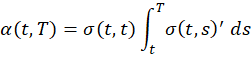
See Björk, “Arbitrage Theory in Continuous Time,” for the derivation.
1.5 Volatility Factors
As a result, any practical implementation of the model must be accompanied by careful estimation and specification of a volatility function. In this discussion we propose the use of PCA to support the estimation of a factor model for the volatility.
Part 2 Estimation using PCA
2.1 Introduction
All code used in the analysis is available upon request. Contact: matia.tamale@yahoo.com.
We will use time series data published by the Bank of England to take the first steps in imposing a volatility structure for our H-J-M model.
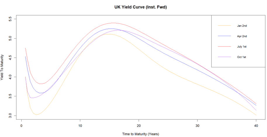
Figure 2.1.1 Graph of nominal instantaneous forward rates for the United Kingdom at the beginning of each quarter (2024).
Source: Bank of England
As the volume of zero-coupon bonds traded in the market is dwarfed by coupon paying bonds, both the zero-coupon yield curve and the instantaneous forward rates must be constructed from coupon-paying bonds via bootstrapping techniques.
The Bank of England publishes its own estimates of instantaneous forward rates constructed from gilts, and it is the nominal series corresponding to 2024 that we use to perform the analysis.
2.2 Data Treatment and Processing
For PCA it is essential that we work with stationary time series. Univariate tests such as the Augmented Dickey-Fuller test as well as multivariate tests were run with the conclusion the series were integrated of order 1. This is exemplified by the autocorrelation function of the 10-year instantaneous forward rate, which exhibits significant persistence. To achieve stationarity, the series were differenced.

Figure 2.2.1 Time series of the 10 year instantaneous forward rate.

Figure 2.2.2 Autocorrelation function of 10 year instantaneous forward rate
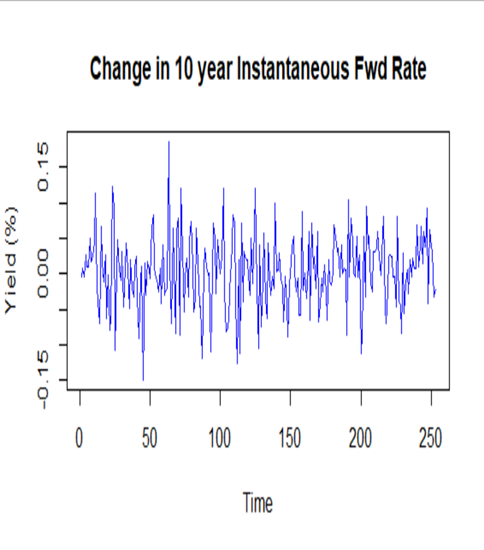
Figure 2.2.3 Graph of the differenced time series
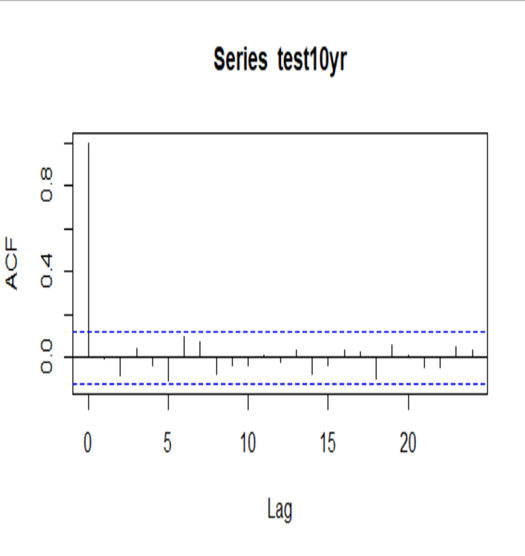
Figure 2.3.4 Autocorrelation function of the differenced data
2.3 Constructing the Variance-Covariance Matrix
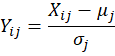
As a result, we can form the resulting differenced data into a matrix. For PCA we must scale and centre our variables to ensure that each of the columns has a mean of 0 and unit variance. It is this centred matrix we then use to construct our empirical Covariance matrix.Hence let our data be arranged in a matrix X where the (i,j)-th element corresponds to the instantaneous forward rate on date ‘i’ with maturity ‘j.’
.
Note: ‘i’ ranges from 2nd January 2024 to 31st December 2024, and j corresponds to a 9-month maturity, followed by a 1-year maturity, with subsequent semi-annual increments thereafter.
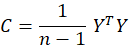

The eigenvectors of the resultant matrix provide the loading vectors of the principal components whereas the eigenvalues relate to the principal component scores.
Note: Computed using the Singular Value Decomposition (SVD) for numerical stability. The process however is algebraically equivalent.
2.4 Intuition gained from results
| Principal Component | Proportion of Variance Explained | Cumulative Proportion | Interpretation |
| PC1 | 88% | 88% | Level |
| PC2 | 5.6% | 94% | Slope |
| PC3 | 3.1% | 97% | Curvature |
| PC4 | 1.3% | 98% |
Figure 2.4.1 A table reporting the results from the Principal Component Analysis
The first principal component has near uniform loadings across all maturities crucially with the same sign, indicating that most of the daily variation is explained by the average level of the yield curve. The second component displays large negative coefficients for short-term maturities and lesser, positive coefficients for longer-term maturities, reflecting slope changes more sensitive to short-end maturities. The third component, with negative coefficients at both ends of the curve and a positive coefficient for maturities in the middle, captures curvature or hump-shaped variations in the yield curve.
The first three components together explain over 97% of the variation in the data, aligning with the empirically observed three-factor model of level, slope, and curvature.
2.5 Conclusion
To finalise one could then go on to explicitly construct a volatility function using the first ‘n’ principal components which would then allow specification of a Heath-Jarrow-Merton type model for interest rates and could be used to simulate paths for rates and price interest rate products.
In practice, however, additional techniques such as the Kalman filter are often employed to handle nonlinearities, particularly given the non-Markovian nature of the term structure. Furthermore, care must be taken when relying on parameters fitted to historical data. Good modelling practice involves using a suite of models, recalibrating regularly, and avoiding reliance on any single framework.
Sources
Heath, D., Jarrow, R., & Morton, A. (1990). Bond Pricing and the Term Structure of Interest Rates: A Discrete Time Approximation. The Journal of Financial and Quantitative Analysis, 25(4), 419–440. https://doi.org/10.2307/2331009
Heath, D., Jarrow, R., & Morton, A. (1992). Bond Pricing and the Term Structure of Interest Rates: A New Methodology for Contingent Claims Valuation. Econometrica, 60(1), 77–105. https://doi.org/10.2307/2951677
Björk, T. (2009). Arbitrage theory in continuous time. Oxford University Press.