This report examines the volatility in Global LNG markets, focusing on the dynamics of supply, demand, and geopolitical influences. It also models price fluctuations and explores the implications for market participants.
(Written in July 2024)
1.1 Overview
In 2022, the volatility of LNG prices surged globally due in part to supply uncertainties stemming from the Russia-Ukraine war, a structural shift in demand as European importers sought alternatives, and the relatively low price elasticity of demand caused by organisational and transport constraints.
The uptick in volatility has presented opportunities for speculators and traders, as more volatile markets often lead to asset mispricing and consequently arbitrage opportunities become more prevalent. Commodity derivative traders must also pay attention to volatility as implied volatility is crucial in the valuation and pricing of several securities used extensively by traders and risk managers to hedge trading positions or market exposure gained through supply and production.
In this discussion, we will first provide a contextual backdrop for Global LNG markets, outlining the key factors shaping its dynamics. We will then analyse potential future developments and the prevailing uncertainties persisting within the market. Following this, we will examine and model the volatility present, exploring its implications for the market and its participants.
2.1 Supply Side
| Nation | Volume (Tonnes) |
| United States | 86,000,000 |
| Qatar | 80,000,000 |
| Australia | 80,000,000 |
Figure 2.1 A table displaying the leading LNG exporters globally (2023)
Source: Shell LNG Outlook 2024
As we move into the second half of 2024, supply is expected to expand at unprecedented levels. U.S. export capacity is projected to nearly double by 2028. Additionally, Qatar’s development of their North Field complex will lead to a significant increase with the initial phase expected to be online in 2025.
A directional view on price will be determined by the traders’ view on the path of demand specifically whether it can keep pace with record supply that is expected to come to market over the following years.
To understand this further we will need to examine global LNG demand its drivers.
3.1 Demand Side
| Nation | Volume (Tonnes) |
| China | 72,000,000 |
| Japan | 66,000,000 |
| South Korea | 44,100,000 |
Figure 3.1.1 A table displaying the world’s leading LNG importers (2023)
Source: RBAC
In 2023, China emerged as the largest LNG importer, surpassing Japan due to a marked increase in Chinese demand coupled with a decline in Japanese imports. In the very short term, we expect Chinese demand to remain strong however there is more uncertainty over the medium term. It is clear we must understand their economic trajectories to take a view on the strength of future demand.
3.2 Chinese stagnation
China is currently experiencing a significant growth slowdown and a housing market crisis. Over the medium term, China’s gas demand is expected to rise, but LNG may prove uncompetitive if elevated price levels persist. Alternatives such as domestic gas and imported pipeline gas could provide suitable substitutes in case of sustained high LNG prices. While a recovery in China would materially impact global demand, this scenario is not widely considered the base case, and the situation remains uncertain.
3.3 Japanese Monetary Policy and its implications
Recent changes in Japanese monetary policy, including the Bank of Japan’s move away from negative interest rates and the abandonment of yield curve control, have yet to demonstrate whether they will be sufficient to stimulate significant growth in Japan, which has struggled with sluggish growth for decades. Consequently, we anticipate that Japanese LNG demand will increase only modestly. Meanwhile, over half of global LNG demand comes from South Korea, Japan, and Europe. In Europe, demand for LNG has expanded significantly in recent years as governments sought to reduce reliance on Russian pipeline gas.
4.1 Volumes & Nature of contracts
The LNG market is set to expand significantly in terms of volumes, but many contracts remain long-term, highly personalised, and slow to adjust. This lack of responsiveness and standardization contrasts with more liquid markets like crude oil. However, as the relatively younger LNG market develops and matures, we expect it to increase in responsiveness and, consequently, volatility.
4.2 Price Uncertainty & Volatility
As discussed, taking a directional view on price proves extremely complex, with many unpredictable factors affecting supply and demand dynamics. Each factor is difficult to predict in terms of magnitude and significance, further exacerbated by the presence of geopolitical threats, which are inherently unforecastable and can cause significant swings in price paths, as observed from the Russia-Ukraine conflict.
A bullish view could be built on a prediction of a Chinese recovery, leading to marked demand growth due to China being a leading importer. Conversely, a bearish view might be driven by oversupply and sluggish global growth prospects. The market is expected to exhibit a wide range of price expectations, influenced by new developments. These conditions, along with the increasing presence of hedge funds and high-frequency traders, are conducive to the heightened volatility we currently observe and expect to continue observing.
4.3 Impact & Significance of volatility
As previously mentioned, volatility is crucial for traders since many derivatives are valued either directly or indirectly off some measure of implied volatility. Writers and buyers of options are typically implicitly long or short volatility, depending on the type of option, strike price, and whether the option is in or out of the money. Therefore, an accurate understanding and forecast of volatility is imperative.
5.1 Modelling Volatility
If you wish to see further detail of the analysis, statistical tests and code used contact me on email (matia.tamale@yahoo.com)
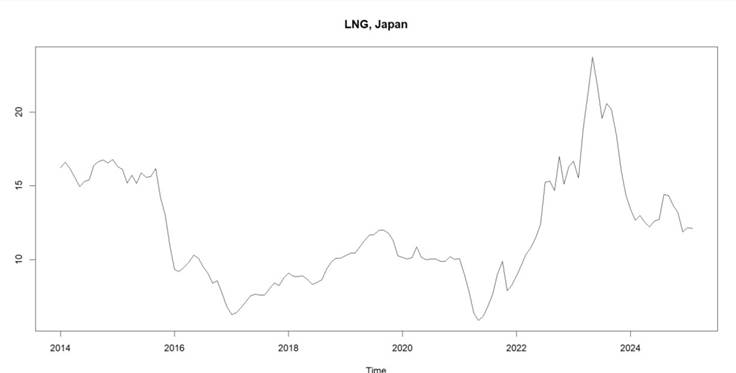
Figure 5.1.1 A time series plot of Japanese Liquefied Natural Gas prices 2014-2024
5.2 Modelling the underlying as an autoregressive process
We focus our analysis now on the LNG, Japan time series above spanning 2014-2024.The series was logarithmically transformed to achieve linearity. Tests for stationarity indicated that the series was integrated of order 1, so the series was differenced accordingly. This led to the estimation of the integrated autoregressive model presented below using ordinary least squares (OLS).
∆𝑦𝑡 = 0.3458 ∆𝑦𝑡−1 + 𝜖𝑡
Note ‘y’ is the natural logarithm of price
‘t’ are monthly increments with t=1 corresponding to January 2014
For a thorough account of this determination, please make contact. We will now proceed with the volatility analysis.
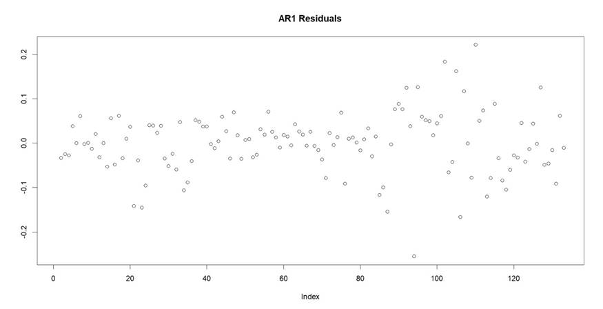
Figure 5.3.1 A plot of the residuals from the autoregression.
5.3 Residuals and Squared Residuals
This residual plot is symmetric around the mean but reveals varying levels of residual variance. While our model is unbiased and explains a substantial portion of the data’s variation, the plot shows periods with consistently low residuals, indicating better accuracy, as well as periods with high variance and larger residuals, which violate the homoscedasticity assumption that most forecasting models rely on. The squared residual plot below provides a clearer view of these fluctuations in residual variance.
Homoscedasticity: The assumption that residuals are independent and identically distributed with constant variance
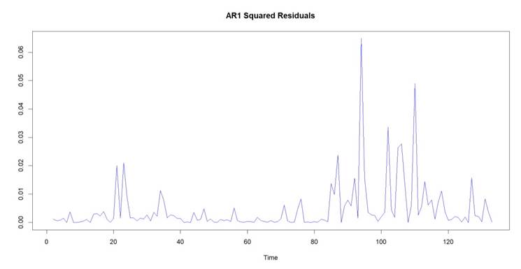
Figure 5.3.2 A plot of the squared residuals.
When we inspect the squared residuals, we observe significant volatility clustering, indicating heteroscedasticity. To formally test for heteroscedasticity, we specify a Lagrange Multiplier test originally proposed by Engle.
5.5 ARCH-LM Test
Test Regression:
\(\begin{align}
\hat{\varepsilon}_t^2 &= \gamma_0
+ \gamma_1 \hat{\varepsilon}_{t-1}^2
+ \gamma_2 \hat{\varepsilon}_{t-2}^2
+ \dots
+ \gamma_k \hat{\varepsilon}_{t-k}^2
+ \nu_t
\end{align}
\)
Test Statistic: NR2
H0: γ1 = γ2 = ⋯ = γk = 0
𝐻A: ∃𝑖 𝑠𝑡. 𝛾i ≠ 0
Distribution under 𝐻0: Chi Squared on 4 degrees of freedom
Critical value: 9.488
Realised test statistic: 62.57
Associated P-Value: 1.66 × 10⁻¹³
Decision: Reject the null hypothesis at the 5% significance level
Figure 5.5.1 An ARCH Lagrange multiplier test for conditional heteroscedasticity
Note ‘ k’ is the order of autocorrelation being tested. Chosen to be 4 in our case
R2 is the coefficient of determination and N the number of observations
We reject the null hypothesis of homoscedasticity and therefore seek to fit a model to remedy this.
5.6 GARCH Model Specification and Fit
The Generalized Autoregressive Conditional Heteroscedasticity (GARCH) model is a stochastic volatility model designed to capture changes in variance over time. It extends the Autoregressive Conditional Heteroscedasticity (ARCH) model by incorporating past conditional variances, allowing for a more parsimonious specification that captures high-order ARCH effects and simplifies the model
In this analysis, the GARCH (1,1) model was estimated using Maximum Likelihood estimation in R.
σ2𝑡 = 0.0002107 + 0.1974523ϵ̂2𝑡−1 + 0.7757036σ2𝑡−1
𝜎𝑡2 denotes the conditional variance at time 𝑡
𝜖̂𝑡2−1 𝑑𝑒𝑛𝑜𝑡𝑒𝑠 𝑡ℎ𝑒 𝑠𝑞𝑢𝑎𝑟𝑒𝑑 𝑟𝑒𝑠𝑖𝑑𝑢𝑎𝑙 𝑓𝑟𝑜𝑚 𝑡 − 1
𝜎𝑡2−1denotes the conditional variance from the previous period 𝑡 − 1
This GARCH (1,1) model can be utilised to gauge current market volatility and update forecasts accordingly, providing valuable insights for pricing derivatives and managing risk.
6.1 Conclusion & Recommendations
During heightened volatility, hedging products such as puts must incorporate increased risk premia to compensate for the higher probability of ending up in the money. Mispricing of these products could be catastrophic and result in substantial losses, making careful pricing essential. Volatility must be monitored attentively.
A recovery in the Chinese economy will provide strong price support, with Chinese policy offering important clues about the market’s direction. Additionally, the speed of the international transition from oil and coal to gas will be critical. A swift transition could lead to rapid structural shifts in supply and demand dynamics, influencing global energy markets and prices. Conversely, a slow transition may result in prolonged periods of volatility and uncertainty, affecting energy investments and policy decisions worldwide.
Sources
IEEFA Global LNG Outlook 2024-2028
https://ieefa.org/sites/default/files/2024-04/Global%20LNG%20Outlook%2020242028_April%202024%20%28Final%29.pdf
IEA Global LNG report Q3 2024 https://iea.blob.core.windows.net/assets/14a61f2b-04fa-4a9d-a78b6c22fc23d5c8/GasMarketReport%2CQ3-2024.pdf
Shell LNG Outlook 2024
https://www.shell.com/what-we-do/oil-and-natural-gas/liquefied-natural-gas-lng/lngoutlook-2024.html
Baringa – Navigating risk: the complexities and challenges of LNG trading https://www.baringa.com/en/industries/energy-resources/energy-commoditiestrading/navigating-risk-lng-trading/
RBAC: China’s LNG Surge: Surpasses Japan as Top LNG Importer https://rbac.com/chinas–lng–surge–surpasses–japan–as–top–lngimporter/#:~:text=China%20imported%20a%20total%20of,production%20and%20pip eline%20gas%20imports.
Hamilton, J.D. (1994). Time series analysis. Princeton, N.J.: Princeton University Press.
Hull, J. (2022). Options, futures, and other derivatives. New York, Ny Pearson.